This is the second post of our series on the analysis of privacy risks with synthetic data from an engineering point of view. In the first post, we introduced the data privacy problem and defined some specific risks to be taken into account. Here, we delve into the technical details. We present some methodologies to actually quantify the risks.

Let’s go back to the scenario that we described in the previous post: starting from an original dataset O we generate a synthetic dataset S with a certain degree of protection in terms of privacy. We want to prevent re-identification of any kind. We therefore want to prevent a possible attacker A, having S at their disposal, from being able to derive sensitive information about real individuals in O. So, first of all, we have to measure how different, or distant, synthetic individuals are from real individuals. The more distant they are, the more difficult re-identification is. We need a reasonable measure of distance between each pair of records (s, o).

Distance between individuals

We are talking about personal data in tabular form that may contain qualitative (categorical features) and quantitative (ordinal features) information. Here is an extract from the popular UCI Adult dataset that well represents this type of data:

How can we measure the distance between two rows in this dataset? We need a similarity coefficient that combines the difference between both types of features. We want the distance to always be between 0 (identical individuals) and 1 (individuals at the maximum distance). For this purpose, the Gower distance is a great solution. Given two individuals i and j, each consisting of p features (the columns of the dataset), we can thus define their Gower distance as

where d_ijk is the distance between the k-th feature and w_ijk is an (optional) weight assigned to the k-th feature. To make things simpler we can consider w_ijk=1 for all features i.e each feature contributes equally to the overall distance, and thus obtain the following simplified formula:

The distance d_ijk is distinct for categorical and ordinal features:

• For categorical features:

• For ordinal features:
  
  where R_k is the range for the k-th feature.

Now that we have a way to calculate the distance between two individuals, we can use it to construct our first privacy metric.

Distance to Closest Record

We aim to verify that the synthetic individuals in S are not a simple copy or the result of a simple perturbation (addition of noise) of the real individuals in O. We can define the Distance to Closest Record for a given individual s in S as the minimum distance between s and every original individual o in O:

DCR(s) = 0 means that s is an identical copy (clone) of at least one real individual in the original dataset O. We calculate the DCR for each synthetic record s in S and plot the resulting values as a histogram to observe their distribution. From such a chart we can quickly obtain a first insight into the overall level of privacy of our synthetic dataset.

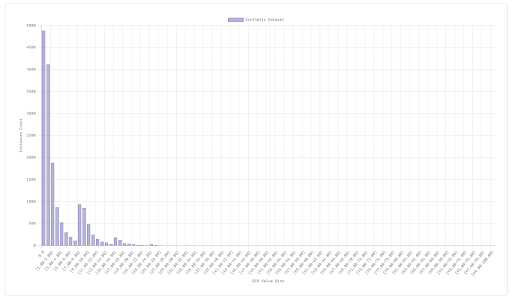
See the initial spike at 0? It means that there are many synthetic instances matching at least one real individual, i.e. many real individuals are copied identical in the synthetic dataset. Not exactly what we would expect from a synthetic dataset that should prevent re-identification of the original individuals. If we get such a histogram, it is wise to stop and examine the situation better. The risk of re-identification could be high. The synthetic data generation process may need to be reconsidered, there may have been overfitting on the original dataset for example.

However, this situation does not always indicate a high risk of re-identification: in some datasets the cardinality “covered” by the features might be so low as not to allow for a sufficiently diverse generation. Let me explain this better with an extreme example: if the original dataset has exactly 4 categorical features/columns and each has only two possible values there would be exactly 16 possible individuals, consequently any sufficiently large synthetic dataset will present identical instances to the original ones.

On the other hand, here’s how a good (in terms of privacy risk) DCR histogram looks like:

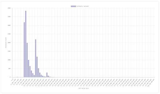
The values distribution is sufficiently far from 0 and notably there is no individual who has a DCR exactly equal to 0, i.e. none of the real individuals are identically present in the synthetic dataset. First test passed, we can carry on with our analysis.

Synthetic vs Holdout

Let’s slightly modify the initial scenario and assume that we have split the original dataset in two sets: one part, the training set T, is used for synthetic generation while the second part, the holdout set H, is kept aside without being used by the generative model. If you have developed machine learning models in the past, this split should be familiar to you.

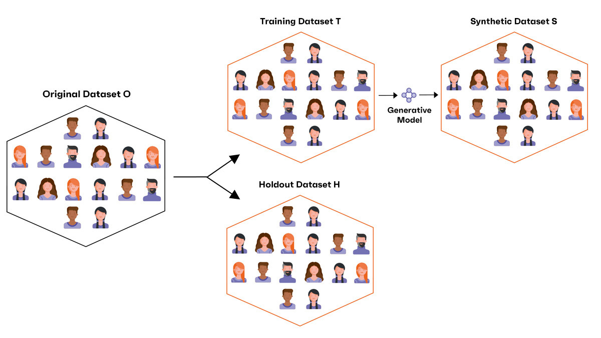
This way, in addition to calculating the DCR between the generated synthetic dataset and the training set as we did before, we can also calculate the DCR between the synthetic and the holdout dataset. Ideally we would like to check that the synthetic individuals are not systematically closer to those in the training set than those in the holdout set. We can again represent these distributions with a histogram.

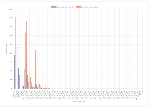
In this example, we immediately notice that the synthetic dataset is much closer to the training set than the holdout. This is not good in terms of privacy. It means that we were not able to generate synthetic instances sufficiently different from the training ones and this results in a high risk of re-identification.

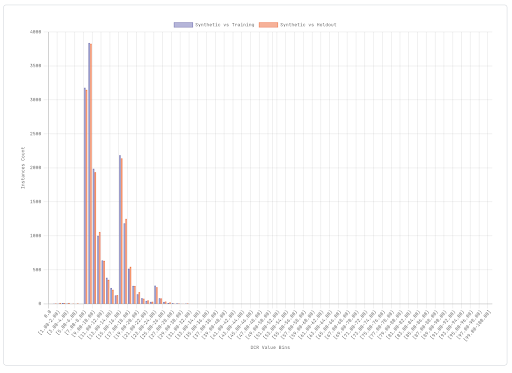
Here instead is a satisfactory histogram. The distribution of distances between synthetic and training instances is very similar (or at least not systematically smaller) than the distribution of distances between synthetic and holdout instances. With T, S and H available, it is virtually impossible to tell which of T and H was actually used to train the generative model. This is a good sign in terms of privacy risk.

We can summarise this metric into a single value that at a glance tells us our level of privacy. Having DCR values for all synthetic instances against both training set and holdout set instances, we can calculate the percentage of synthetic instances that are actually closer to a training set instance than to a holdout set instance. In the best cases we obtain a percentage close to (or below to) 50%: this means that the synthetic dataset does not provide any information that could lead an attacker to assume whether a certain individual was actually present in the training set.

This first set of metrics already provides us with a lot of useful information on the level of privacy risk of our synthetic dataset. Stay tuned for the next post of the series, we’re going to analyse further methodologies to check the risks of more sophisticated attacks.