Have you ever worked on real-life data science projects? If yes, you may be familiar with imbalanced datasets. If not, you might encounter them soon. In this blog post, we discuss the concepts and the issues related to imbalanced datasets and present two techniques to augment your dataset when you encounter such an issue.

Training models on an imbalanced dataset

An imbalanced dataset is an annotated dataset where the distribution of the target labels is very uneven, i.e. a label might appear much less frequently than the rest. This issue often affects datasets ranging from credit scoring to predictive maintenance, where the predictive target refers to situations that rarely happen. Even though we refer to structured data in this post, the same concepts are valid for non-structured data such as images or text.

Training a classification model on an imbalanced dataset makes things complex from a parametric optimisation perspective. For example, if we optimise our parameters using a gradient descent algorithm, the contribution to the update from the minority class would be minimal or even non-existent for many descent steps. How can we tackle this problem? The most natural operation to balance imbalanced datasets is either by undersampling the majority class or by oversampling the minority one.

Undersampling (or downsampling)

Undersampling corresponds to discarding many points from the majority class according to a chosen strategy like random. This process aims to make the distribution of the target label more even, thus making minority examples contribute more during the training process. One significant limitation associated with undersampling approaches is that we may discard good data, which is not always desirable, especially when training big models. One can go beyond simple random undersampling by adopting more sophisticated strategies, such as those implemented in the imbalanced-learn library. Following such techniques , you can effectively select and remove points from the training set that have the lowest influence on the model performance.

Oversampling (or upsampling)

On the other hand, oversampling creates additional points representing the minority class, introducing new data that was not present in the original dataset. These points are, by definition, synthetic as they are generated by an algorithm. Over the years, researchers proposed many algorithms to perform the oversampling task, the most popular being SMOTE. The original SMOTE article was published in 2002, and since then arguably no other method has been as popular.

What is SMOTE oversampling?

SMOTE stands for Synthetic Minority Over-sampling Technique. To generate a new point, SMOTE first chooses a random point from the minority class and then randomly selects one of its N-nearest neighbours. The number of neighbours N are defined by the user. Once a random neighbour is selected, a synthetic point is generated by creating a weighted average between the original minority example and its neighbour. You can see a visual representation of the SMOTE algorithm in Figure 1.

The procedure to generate synthetic points with SMOTE is quite clever and effective; however, it comes with significant limitations. First of all, finding the nearest neighbours requires the definition of a robust distance metric which is not trivial, especially in the presence of nominal data. Second, by performing this operation, we are overpopulating certain regions of the feature space with minority labels, possibly affecting model calibration. A model trained on a dataset balanced using SMOTE might be overconfident about minority points.

An alternative approach: generative models such as VAEs

An alternative to SMOTE is to obtain synthetic points using generative models such as Variational AutoEncoders. Generative models have demonstrated enormous potential when handling complex data distributions during the last few years. Their success at generating realistic data makes them a new paradigm to solve dataset oversampling.

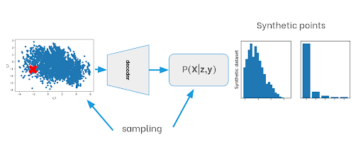
Generative models are trained to learn joint probability distributions of the dataset we are dealing with. This information gives us the possibility of sampling new points that are realistically distributed, and ideally, this would allow us to sample realistic minority examples.

For example, Variational AutoEncoders are designed to learn the following conditional joint distribution:

X represents the points we want to sample, usually defined as a combination of features. For example, if we talk about a dataset describing individuals, sampling from X means calculating the probability of a certain age associated with a particular professional background and education level.

The joint probability is conditioned to y, the target label, and to z, a latent variable used to represent the problem in a simplified space. The variable z allows us to define a sampling strategy, as shown in Figure 2 . Since we know that z is normally distributed we can easily sample realisations that can be fed to the decoder to finally obtain samples from the joint conditional distribution P(X|z,y).

Learning this simplified representation z helps overcome the limitations above by learning robust distance metrics, especially for mixed data types. Furthermore, it helps reduce label imbalance by oversampling minority and majority classes in regions of the latent space where the imbalance is less pronounced. A discussion of oversampling strategies based on the latent variable z will be presented in the next blog post.

To be continued: a practical example

With this post, I wanted to introduce the concept of using generative models to perform minority oversampling for an imbalanced dataset as opposed to standard techniques such as SMOTE. In the next part, we will discuss a practical example based on a popular credit card fraud detection dataset affected by an important label imbalance. Stay tuned!