In previous posts we discussed the importance of associating machine learning predictions with robust uncertainty estimates. We discussed here how traditional machine learning can be affected by poor model confidence estimates and how it is possible to improve them using post-hoc calibration.

In this post we will discuss a specific family of machine learning models which are designed to incorporate uncertainty by design: Bayesian models. We will also present an example on how to implement a Bayesian neural network using the PyMC3 library.

What are Bayesian models?

The idea behind Bayesian models is to treat model parameters as conditional distributions with respect to the evidence represented by the problem data. This kind of approach differs from traditional machine learning because instead of determining point estimates for the model parameters we are now trying to represent them using distributions we can sample from. This approach is of course better suited to represent model uncertainty associated with the data used to train it.

This family of statistical models is called Bayesian because it defines the quantity of interest, the probability distribution of the model parameters conditioned to the problem data p(θ|data), using Bayes’ theorem. This theorem can be used to calculate a probability associated with a certain quantity based on prior knowledge we have about the same quantity and it reads

The posterior p(θ|data) is expressed as a function of the following terms

• p(data|θ) is the likelihood term corresponding to the parameterization of the data represented by the model itself. By maximizing this probability we would perform Maximum Likelihood Estimation obtaining a point estimate.
• p(θ) or the prior which corresponds to our initial belief on how the parameters are distributed. We can for example initially assume our model parameters to be gaussian distributed.
• p(data) or the evidence, corresponding to the joint distribution of the problem data, for example the input output distributions X,y in traditional supervised machine learning problems.

The posterior is the conditional probability distribution we are looking for. Unfortunately a closed solution of the equation above cannot be found very easily because of the inherent complexity of the evidence term, however there are techniques that can be used to tackle this problem numerically. One approach is via Monte Carlo sampling in particular through Markov Chain Monte Carlo, which allows sampling from the posterior distribution at a very high computational cost.

Another approach is represented by Variational Inference which introduces assumptions about the posterior probability making the problem more tractable. In this kind of approaches instead for the original posterior probability we looking for a simplified distribution q that minimizes the KL divergence

The distribution q is assumed to belong to a certain family, for example Gaussian, and to be parametrized by Φ. In this way we can set up the problem as finding the value of Φ that minimizes the KL term.

In the example below we show how to fit a Bayesian Neural Network using a Variational Inference approach, the ADVI which solves the problem above using model gradients to speed up convergence.

Fitting a Bayesian Neural Network with PyMC3

To show the main concepts behind Bayesian models we take the same credit risk problem we analyzed in the previous posts and we implement it using a popular probabilistic programming library, PyMC3. This library includes a number of probabilistic solvers and makes use of Theano for the definition of neural networks.

The following snippet (taken from here), shows how a Bayesian neural network can be created in PyMC3:

import pymc3 as pm
import pymc3
from pymc3.theanof import set_tt_rng, MRG_RandomStreams
set_tt_rng(MRG_RandomStreams(42))

import theano.tensor as T
import theano
floatX = theano.config.floatX

def construct_nn(ann_input, nn_labels):
  n_hidden = 4
  # Weight inizialization
  init_1 = np.random.randn(X_train.shape[1], n_hidden).astype(floatX)
  init_out = np.random.randn(n_hidden).astype(floatX)

  with pm.Model() as neural_network:
    # Prior distribution for input weights
    weights_in_1 = pm.Normal('w_in_1', 0., sd=1., shape=(X_train.shape[1], n_hidden),
                            testval=init_1)

    # Activation hidden layer
    act_1 = pm.math.tanh(pm.math.dot(ann_input, weights_in_1))

    # Prior distribution for output weights
    weights_1_out = pm.Normal('w_1_out', 0., sd=1., shape=(n_hidden,), testval=init_out)

    # Output activation
    act_out = pm.math.sigmoid(pm.math.dot(act_1, weights_1_out))

    # Binary classification -> Bernoulli likelihood
    out = pm.Bernoulli('out', act_out, observed=nn_labels, total_size=y_train_en.shape[0])
  return neural_network


nn_input = theano.shared(X_train)
nn_labels = theano.shared(y_train_en)
neural_network = construct_nn(nn_input, nn_labels)

Here we initialized the architecture as a neural network with one hidden layer and specified what are the priors that we want to use (a normal distribution for each weight). In this particular example we did not include the presence of a bias term in each layer. The choice of the prior can really affect the final model however there is no fixed rule on how to determine them.

The neural network defined above can be fit using the following command where we specify the solver to be used (ADVI):

with neural_network:
  approx = pm.fit(n=25000, method=pm.ADVI())

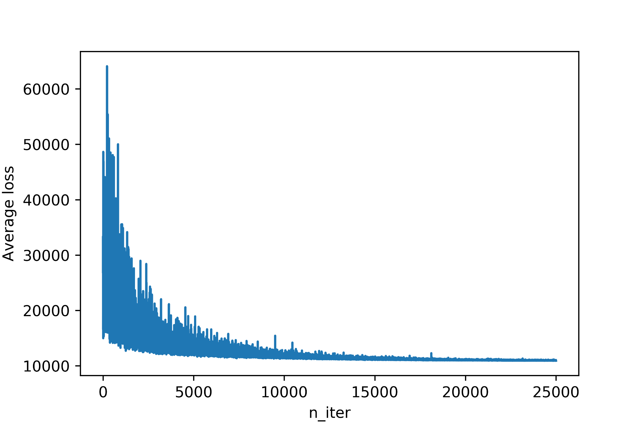
As we do for traditional machine learning problems we can make sure the fitting process has converged by checking the loss function:

Even though ADVI is considerably faster than Markov Chain Monte Carlo sampling the computational costs are much higher than traditional Maximum Likelihood Estimation methods and can become almost prohibitive for more complex architectures.

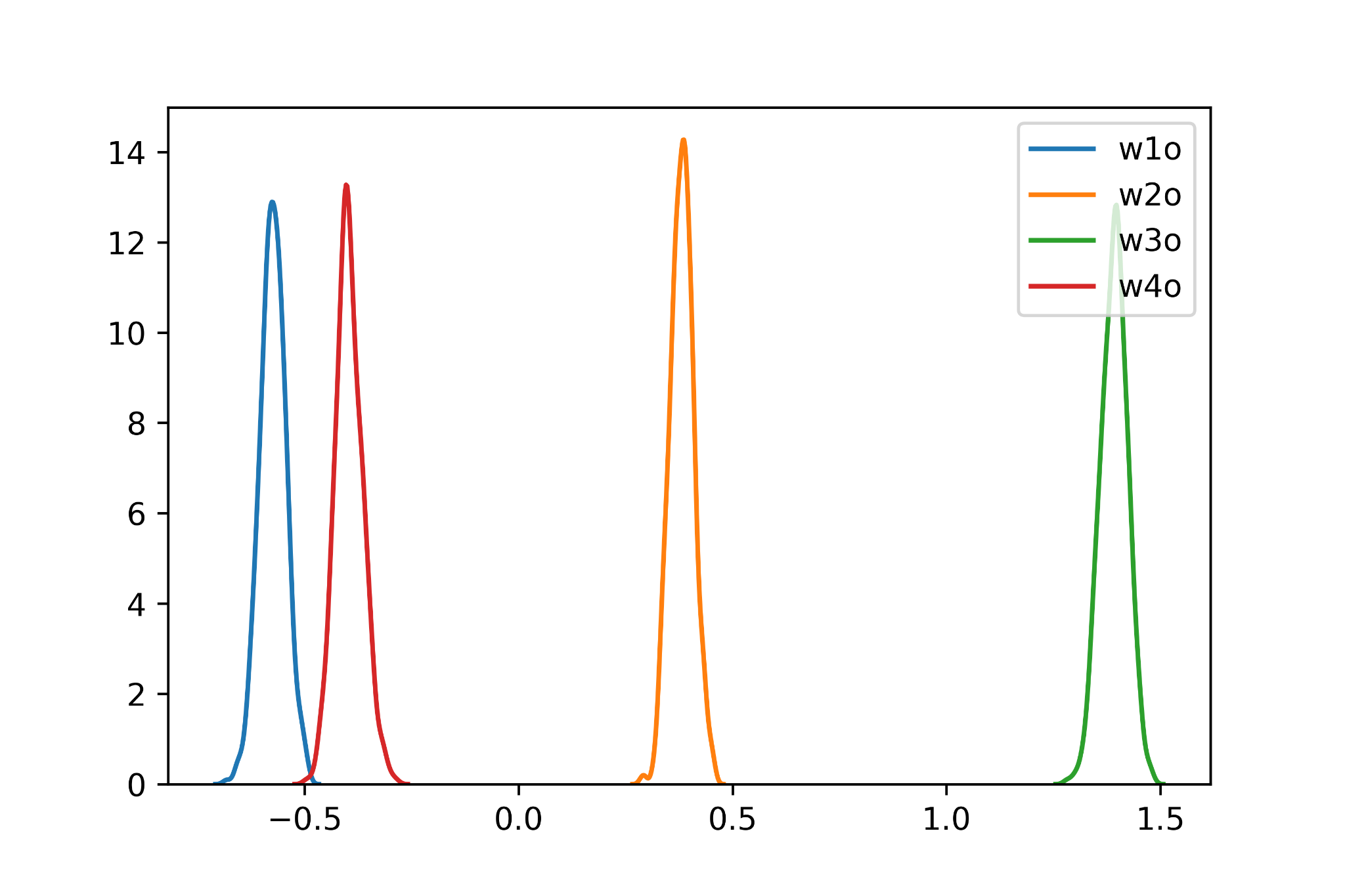
Once the Bayesian network is fitted we can check the distributions associated with each weight. For example the following plot shows the four weights connecting the hidden layer to the sigmoid neuron

The distributions are Gaussian since we are using an approximation to find our posterior and their standard deviation should incorporate the uncertainty present in the training data.

To make new predictions we need to sample again by taking a new input and by randomly sampling the neural network weights until our output converges. Below such output is show in the form of a probability distribution:

As mentioned above, instead of having a point estimate for our model confidence we now have a probability distribution which should be more statistically robust with respect to the aspects discussed in the first post of this tutorial.

It is important to note that Bayesian models are computationally expensive not only at training time but also during inference because we need to sample our model outputs enough times to achieve statistical convergence. This could cause an almost insurmountable obstacle for use cases where large model throughput are required, making this family of methods less appealing.

I hope this third chapter of our tutorial was interesting and useful for you. If you haven’t yet, you can also take a look at the previous tutorial blogpost on how to deal with uncertainty in Machine Learning problems in practice and a practical example of model calibration with a credit risk assessment model. Hope you enjoy them, and stay tuned through our newsletter for the final part of the series in the coming weeks!