This post is the second of a four-part series of didactic articles on uncertainty quantification in Machine Learning written by Dr. Luca Gilli. The current article introduces the readers to the basics of machine learning model calibration with a practical example of a credit risk assessment AI model.

In a previous post we discussed uncertainty quantification in machine learning and about the fact that uncertainty is usually incorporated in a single quantity, the model confidence. The main issue with the singular metric is that the model’s confidence in its own predictions is very often not statistically robust. This happens when the model’s confidence in a certain prediction is not reflected by a similar accuracy when checking its correctness with new data. Studies have demonstrated that this issue is particularly important for some types of neural networks.

The robustness of a model’s confidence is crucial for a decision support system based on a machine learning model, where a user has to decide whether to adopt or discard a model recommendation. In this post I would like to show how to assess and improve model calibration using scikit-learn. Let’s use a toy ML model to calculate credit risk of a given individual. We used a dataset containing historical loan data from the LendingClub and we built a model to predict the probability whether a certain individual will default the loan that they are applying for. In this notebook you can find how this particular classifier was built (using Keras) and trained.

After developing a model, one of the first objectives when evaluating it is to determine whether the model is calibrated or not. To do so we can make use of a calibration curve, also known as reliability diagram. For a given test set, this curve is obtained, first by dividing the corresponding predicted probabilities into bins, and then by calculating for each bin the fraction of true positives. This tells us about the real accuracy for a certain model confidence.

The scikit-learn.calibration module contains a calibration_curve function that calculates the vectors needed to plot a calibration curve. Witha test dataset X_test, the corresponding ground truth vector y_test, and a classifier clf, we can construct the calibration curve using the following lines:

from sklearn.calibration import calibration_curve

prob_pos = clf.predict_proba(X_test)[:,1]
fraction_of_positives, mean_predicted_values = calibration_curve(y_test, prob_pos, n_bins=50, strategy=’quantile’)

Here we specified the number of bins characterising the curve and that the width of each bin should be calculated using a quantile strategy, by forcing each bin to have an equal number of points. y_test are the test set labels, while prob_pos are the probabilities outputted by the model for a desired class. The resulting curve is shown in Figure 1.

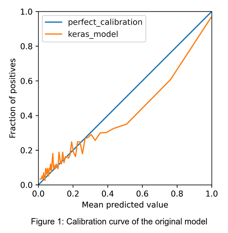
The orange line is the calibration curve we just calculated while the straight blue line corresponds to a perfect calibration. The areas where the calibration curve is below the perfect calibration line are areas where the model is said to be over confident. Conversely when the calibration curve is above the line the model is under confident. What is a practical implication of a model over/under confidence? For the toy problem in question the curve shows that we have an over confident model and that we might be accepting loan applications too conservatively.

How can we improve model calibration when we have uncalibrated classifiers? Scikit-learn comes again to our help with the CalibratedClassifierCV class that can be used to fit a calibrated classifier on top of an original one. Scikit gives the option of using two popular calibration techniques, the sigmoid and the isotonic calibration methods. The sigmoid method (also known as Platt scaling) passes the model output to a sigmoid function whose parameters are fitted to minimise the discrepancy between the model output probability and the training labels.

The isotonic approach is similar but instead of a sigmoid function it uses an isotonic regression. Choosing the right calibration method is not trivial and it depends a lot on the type of problem. Sigmoid calibration works better when we have S-shaped calibration curves.

We can fit a calibrated classifier using the following few lines of code. Since the model is written in Keras we used the KerasClassifier wrapper from tf.keras.wrappers.scikit_learn to make it compatible with the scikit-learn API.

from sklearn.calibration import CalibratedClassifierCV

calibrated_clf = CalibratedClassifierCV(keras_wrapped, method='isotonic', cv= ‘prefit’)
calibrated_clf.fit(X_val, y_val)

Here we specified that we use the isotonic approach and that we are providing a classifier which has been already trained. In this case the calibration function needs to be fit on an hold-out validation set. Using the calibration_curve function on the calibrated classifier allows us to obtain the calibration curve for the test set shown in Figure 2.

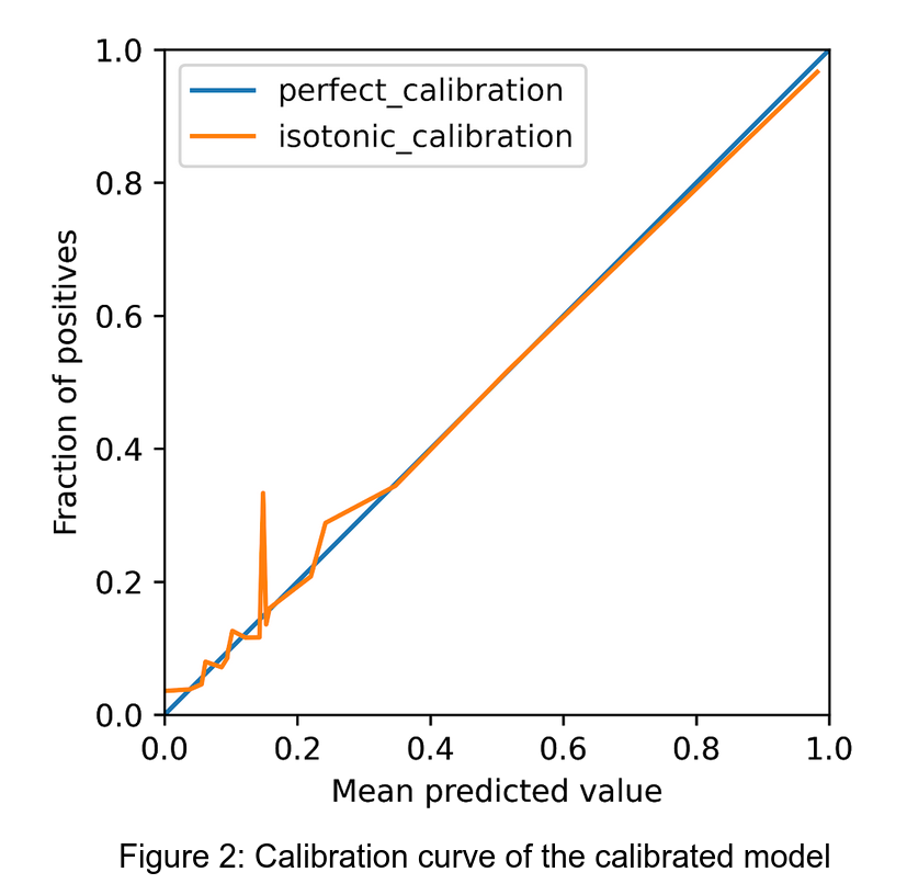
We can immediately notice the improvement compared to the original calibration curve. A potential issue with calibration techniques is that they can be still affected by overfitting with respect to the dataset used to fit the calibrated classifier. In this case the validation set used to calibrate the model belonged to the same distribution as the test set. In general maintaining model calibration with real time data is a non trivial task.

A calibrated model can really improve the usefulness and trustworthiness of a machine learning tool when used as a decision support system. By using robust confidence intervals we can avoid discarding correct recommendations or accepting wrong ones.

In this tutorial we saw how model calibration can be used to improve trust in ML models. In the previous post, we discussed on how to deal with uncertainty in practice and in my next post, I will introduce Bayesian Neural Networks as an alternative way to deal with ML uncertainty. Watch this space!